One important reason for the current, low discovery rates is that a significant part of mineral exploration expenditures is spent in the wrong locations. Often on ‘advanced’ projects that did not work in previous cycles, or simply by looking at known mineral occurrences, and exploring around these locations, in an attempt to find more. While this ‘inside-out’ approach historically led to good results, there are very few remaining ore bodies that can be found by using this approach. Looking ‘from the outside in’ is necessary, if companies want to increase the odds of discovery.
Several months ago, we wrote about the Exploration Search Space, in an attempt to give more visibility to that important concept, which will be key for improving discovery rates. New search spaces regularly open up, often because of new technologies, datasets and research. Another important concept that can help raise the odds of discovery is ‘outside-in’ exploration, a different approach from the more common ‘inside-out’ workflow. These concepts should be used together, across the different scales that are covered during mineral exploration.
Inside-out exploration
There used to be a time when ore bodies were mostly found by looking ‘from the inside out’, essentially by prospecting. Explorers/miners basically looked for (direct expressions of) significant mineralization at surface. They would then try to follow these possible ore bodies into the subsurface, to understand the dimensions, geometry, grades and recovery potential, while actively mining at the same time. This inside-out approach has been used for millennia. The Romans were absolute masters at it, and the majority of mining districts in the southern half of Europe have evidence of mining activities dating back to the Roman Empire. For example, archeological finds of Roman activity (as well as near-surface mine workings) were unearthed at many modern mines in the Iberian Pyrite Belt.
There are still plenty of ore bodies to be discovered close to, or even at the surface, which are not very obvious when applying the usual exploration methods and technologies. Regular discoveries of deeper ore bodies occur in brownfields settings, but greenfields exploration continues to mostly be an activity that helps find near surface ore bodies. There are plenty deposits left to find, of which a small portion is exposed, that is part of a much larger ore body. One recent success story where this was true is Filo del Sol.
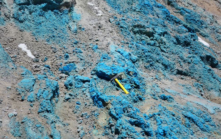
Cu oxides in outcrop at Filo del Sol
While opportunities like that still exist, they are much less common than several decades ago, or located in places with significant ‘above ground’ problems. One way to recognize outcropping deposits in good locations is through the use of modern technologies that augment geologists. For example, with tools that allow geologists to look beyond the visible part of the light spectrum, such as hyperspectral imagery, handheld infrared spectrometers, or even with a UV lamp. Hesperian Metals picked up one such project recently, a high grade tungsten bearing skarn with abundant scheelite, hiding in plain sight, in an old mining camp in SW Spain. But these opportunities logically get fewer and further between, with time.
Global scale
To raise the odds of making greenfields discoveries in this day and age, it no longer makes sense to start working in a location of known mineralization and gradually expanding beyond that. A better approach is an ‘outside-in’ exploration workflow, which starts with understanding the big picture overview. It is particularly important to grasp the structural context and geological setting of a large region that is considered for exploration, before selecting a smaller area within it, and focusing on the relevant aspects of the geology of that area in more detail; a workflow for progressive volume reduction of the region that is being explored, using the most appropriate methods and data for each particular scale.
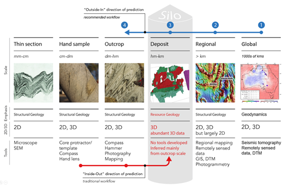
Figure that compares inside-out & outside-in exploration. Adapted from Cowan (2020), to include the important global scale
During the first step (global/continental scale), it is useful to understand the big picture geological settings of different regions around the globe, and their tectonic history, including aspects like the supercontinent cycle and the distribution and geometry of cratonic blocks and smaller blocks of thick lithosphere. The reason that these aspects of the geology are so important is because the distribution of mineral deposits is far from random. Research published in recent years shows that the vast majority of several types of ore deposits (particularly the largest ones) occur at the edges of blocks of thick lithospheric mantle, which are more rigid and buoyant than areas of continental crust that have a thinner lithosphere. Perhaps the clearest example that metal distribution is not random is the statistical representation of sediment-hosted Cu and Pb-Zn deposits by Hoggard et al (2020 – see figure below). Research and publications by Graham Begg (2010), David Groves (2020), and others have also clearly shown the importance of boundaries of blocks of thick lithosphere, for many deposit types.
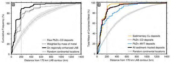
Statistical representation of distance of several sediment-hosted deposit types, from edges of blocks of thick lithosphere (Hoggard et al., 2020)
These rigid blocks are the main building blocks of tectonic plates. Their movements relative to each other largely determine where orogenies, rifts and major strike-slip fault zones occur. The supercontinent cycle helps to understand how these blocks have moved over time, and the processes that drive these movements. Thanks to several geophysical techniques, in many regions across the globe we now have a reasonably good idea about where the edges of thick, rigid lithospheric blocks are found. This is a great aid in determining where to best focus exploration efforts for specific deposit types.
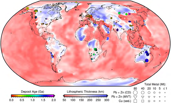
Distribution of major sediment-hosted deposits, overlain on map of depth of lithosphere-asthenosphere boundary (Hoggard et al., 2020)
While this knowledge is incredibly useful, the main geological, geochemical and geophysical datasets that help determine where these edges are, have a very low resolution. Areas that appear to be in a favorable geologic setting are typically >1000 km long, by 100s of kms wide. Exploration companies then need to decide which ground to pick up along these lithospheric boundaries, and select areas that have a reasonable size, that can be explored effectively in the field.
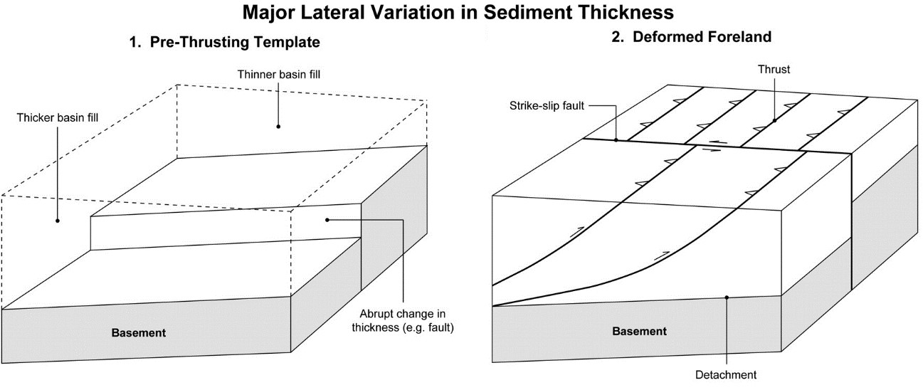
Transcrustal structures
At this stage in the exploration workflow, it is important to select areas along/adjacent to the most likely pathways for fluids and magma’s through the crust. Major, transcrustal structures (and often their intersections), near the edges of blocks of thick, rigid lithosphere, should play an important role during the regionally focused phase of exploration. The problem is that it is difficult to recognize the majority of these ‘vertically accretive structures’, due to their cryptic surface expression (McCuaig & Hronsky, 2014).
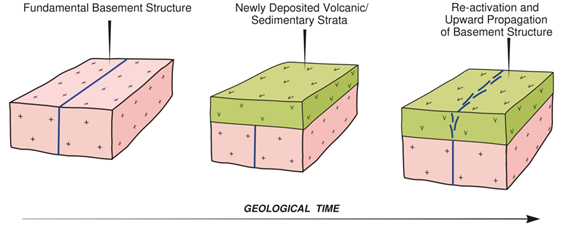
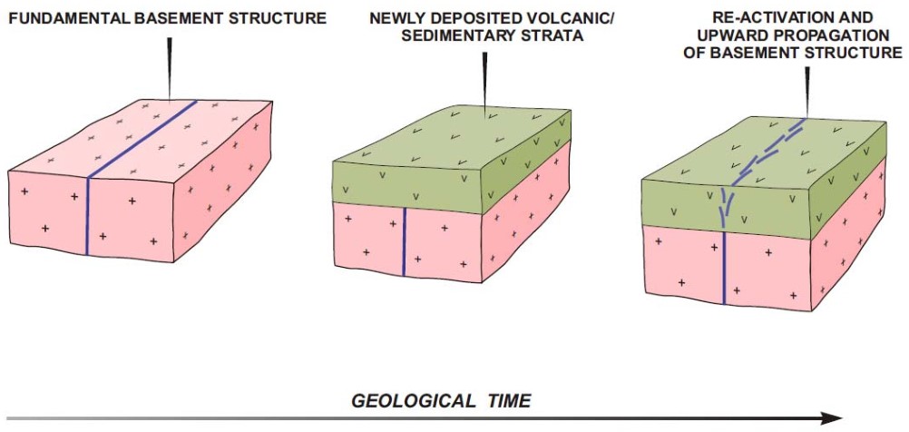
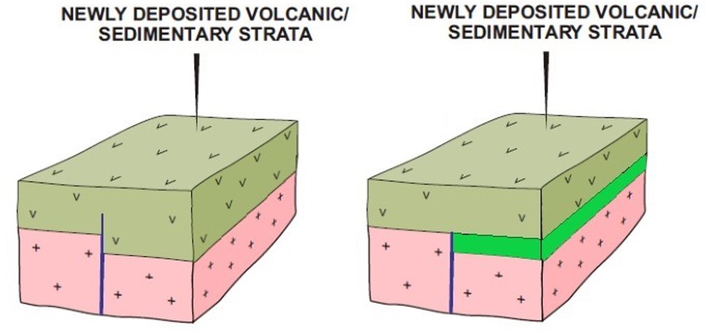
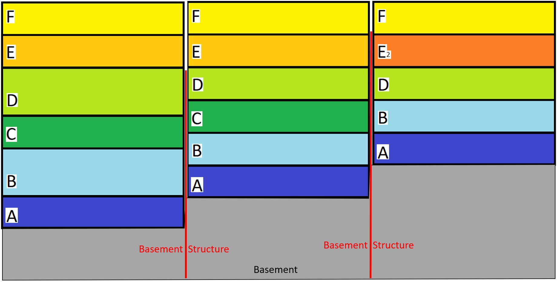
Schematic illustration of vertically accretive structures (McCuaig & Hronsky, 2014)
To find them, it is important to look at the right scale and use the right datasets, which provide a regional perspective. It is impossible to differentiate most of them in the field. Recognizing these crustal scale structures may well be the least effective step in the current exploration workflow, a challenge for which the industry does not yet use a consistent, proven method. Improvements in the ability to accurately map these structures would provide a significant contribution to a necessary increase in future discovery rates.
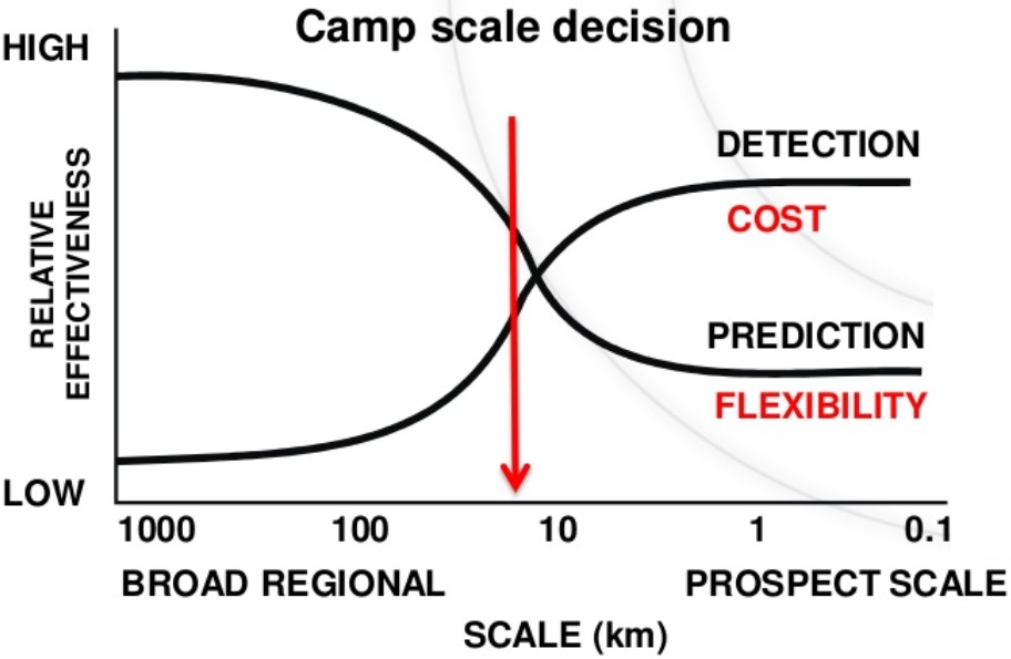
After this important step in the workflow, the ‘camp scale decision’ has to be made, and ground is typically claimed. From that moment onward, exploration expenditure goes up, while flexibility goes down. If the camp-scale decision leads a company to an area that is not along or adjacent to a transcrustal structure, those higher expenditures are generally wasted.
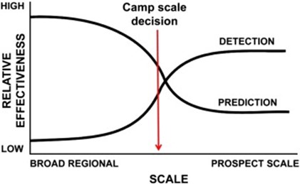
Relative effectiveness of predictive vs. direct detection technologies, across various scales of the exploration workflow (McCuaig et al., 2010)
Some countries have large regional ‘pre-competitive’ geophysical datasets that can help with this step (prime example: Australia). There are clear success stories of targeting based on anomalies in these datasets, such as the discovery of Olympic Dam. But in recent years, these successes are the exception, not the rule. At a global level, the availability of regional geophysical datasets is quite sparse, their resolution is typically low, and acquiring new datasets over large regions comes at a significant cost. While they will continue to play an important role during the early stages of exploration, particularly in areas where the targets are under (undeformed) cover, their limited availability and high cost restrain the widespread use for exploration around the globe.
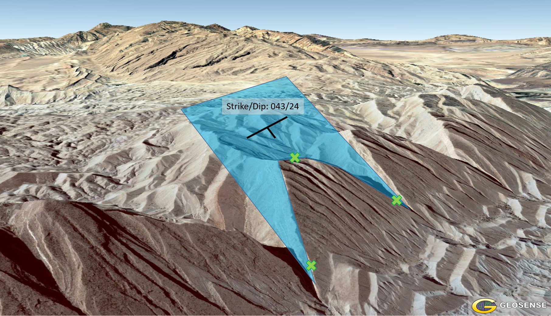
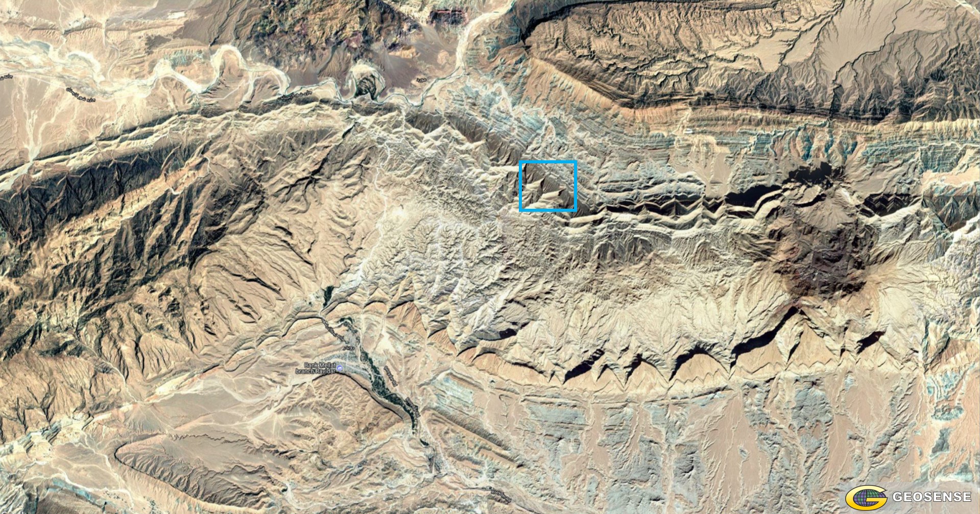
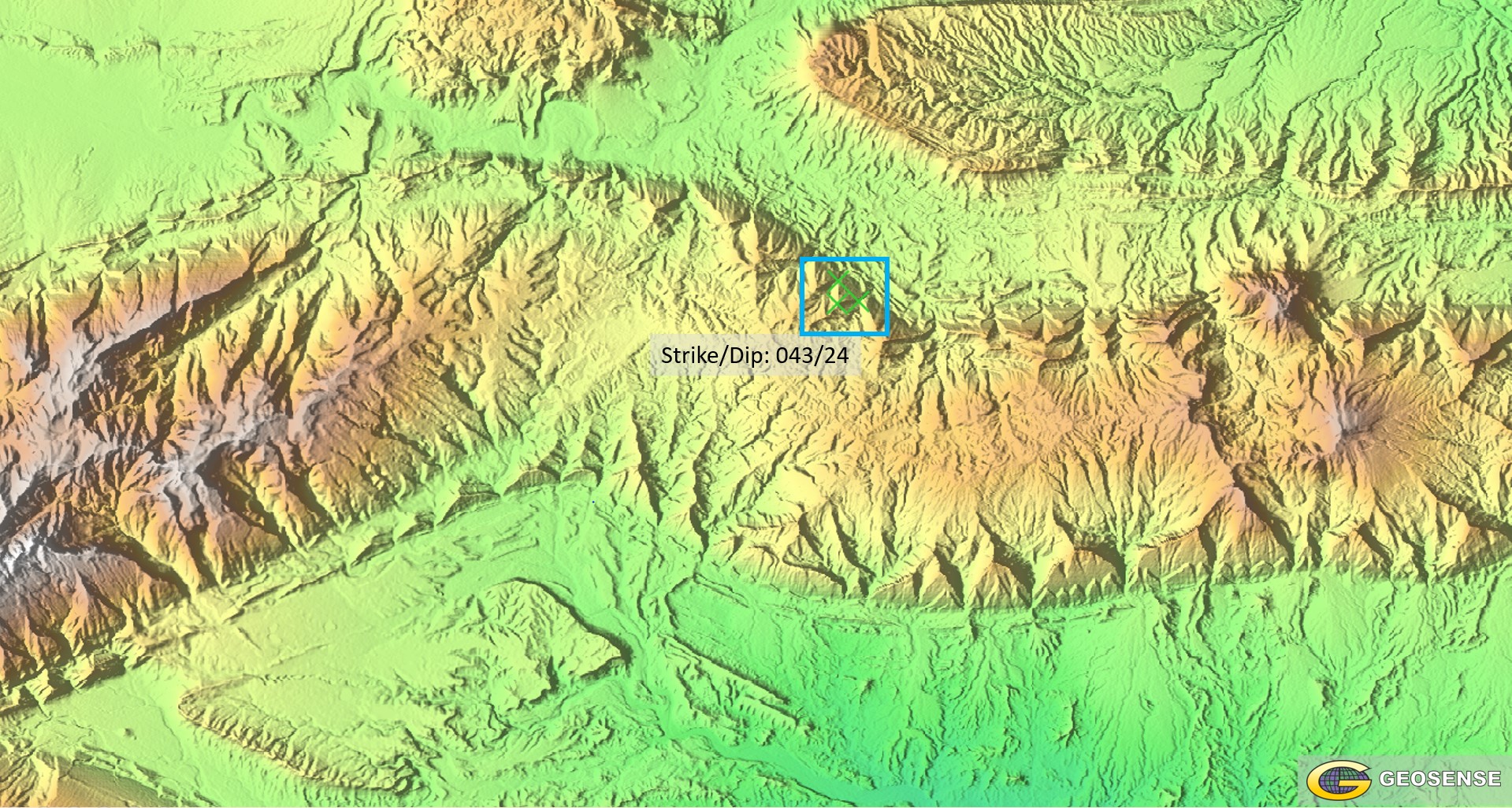
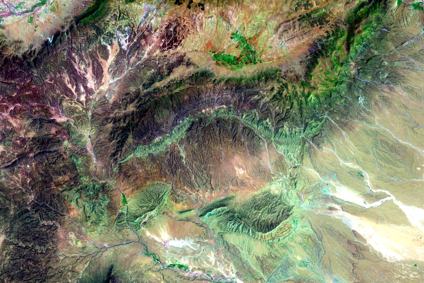
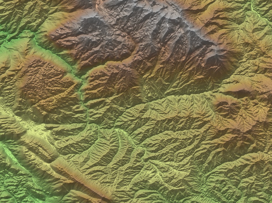
Geological remote sensing
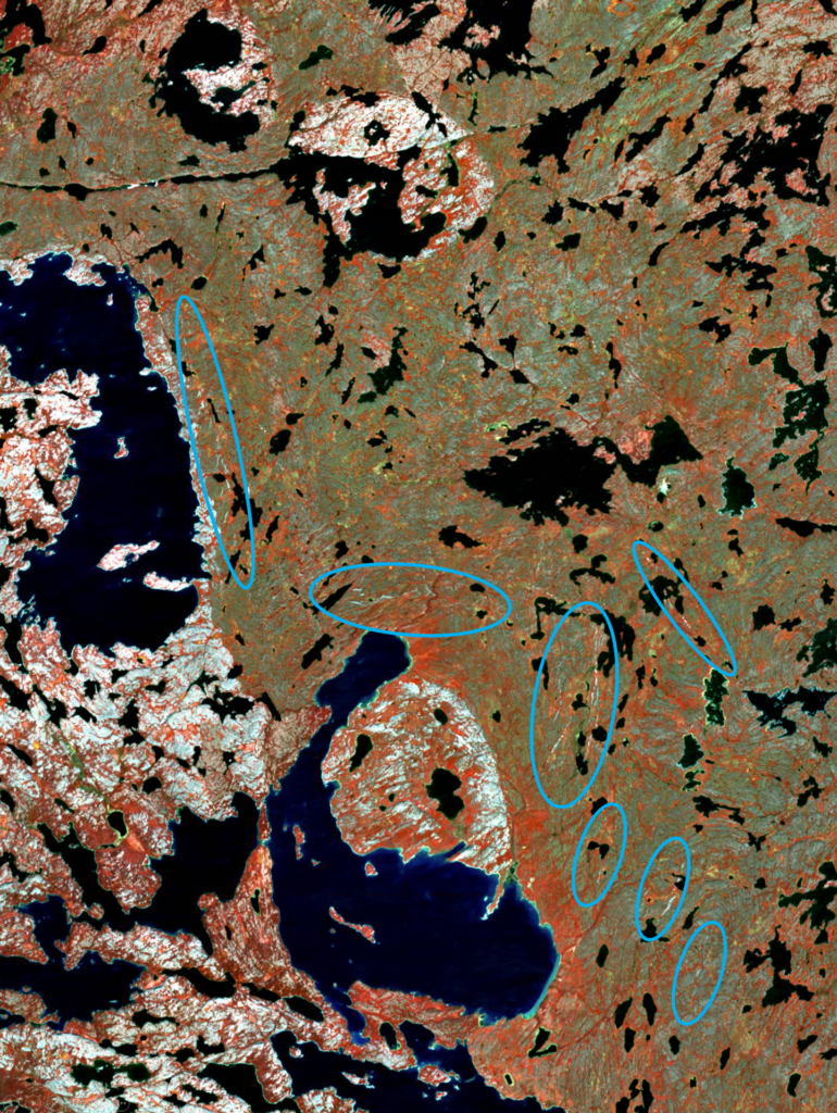
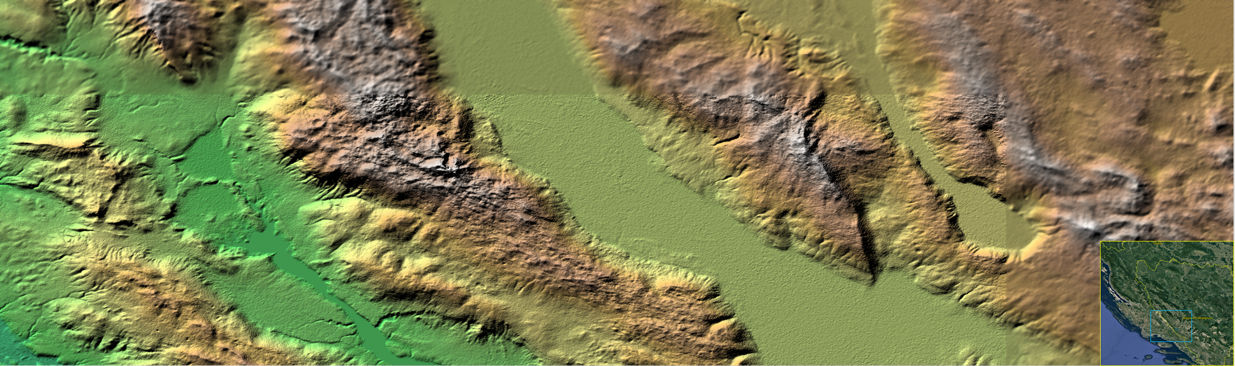
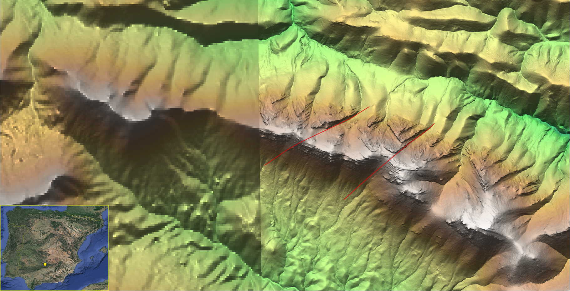
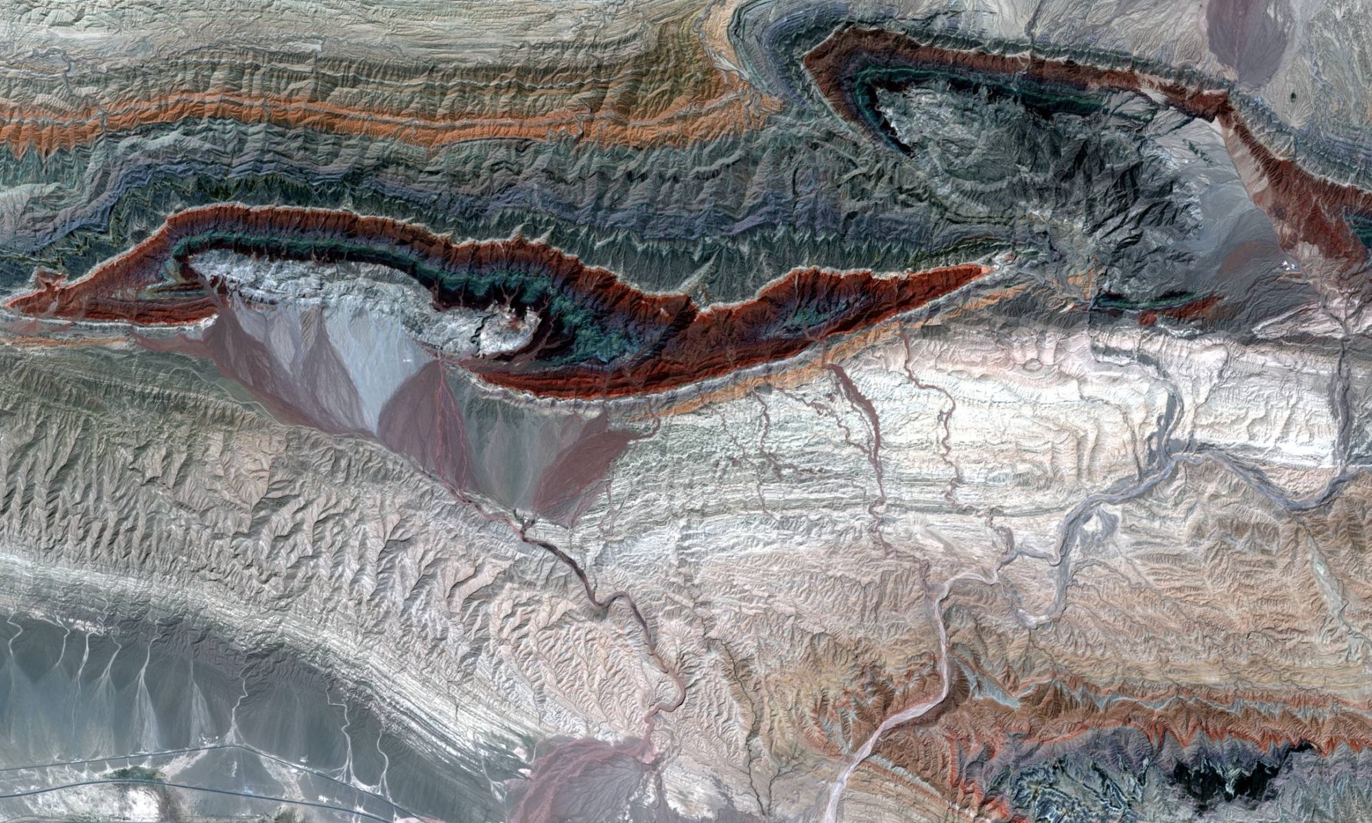
Geological remote sensing is currently the only method that uses datasets that are consistent across the relevant scales for making the camp-scale decision (and beyond), and available across all continents. The two most relevant datasets, which can be used for mapping the geology at surface, are multispectral imagery, and Digital Elevation Models (DEMs). Good quality multispectral satellite imagery (up to 10m spatial resolution), and DEMs (up to 30m spatial resolution) can be downloaded for free from different sources. With these datasets, structural geologists who are specialized in photogeology at different scales, and in different tectonic settings, are able to recognize crustal scale structures in many regions, and map their surface expression in significant detail. We wrote about mapping these fault zones several years ago, and keep studying them, to improve our ability to recognize and map these transcrustal structures and our understanding of the processes that drive their activity. This includes processes that occur in the mantle, which influence how rocks in the upper part of the continental crust deform. Accurate interpretations of transcrustal structures allow explorers to zoom into the most prospective districts of a metallogenic belt, along the edges of rigid blocks of thick lithosphere.
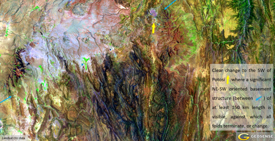
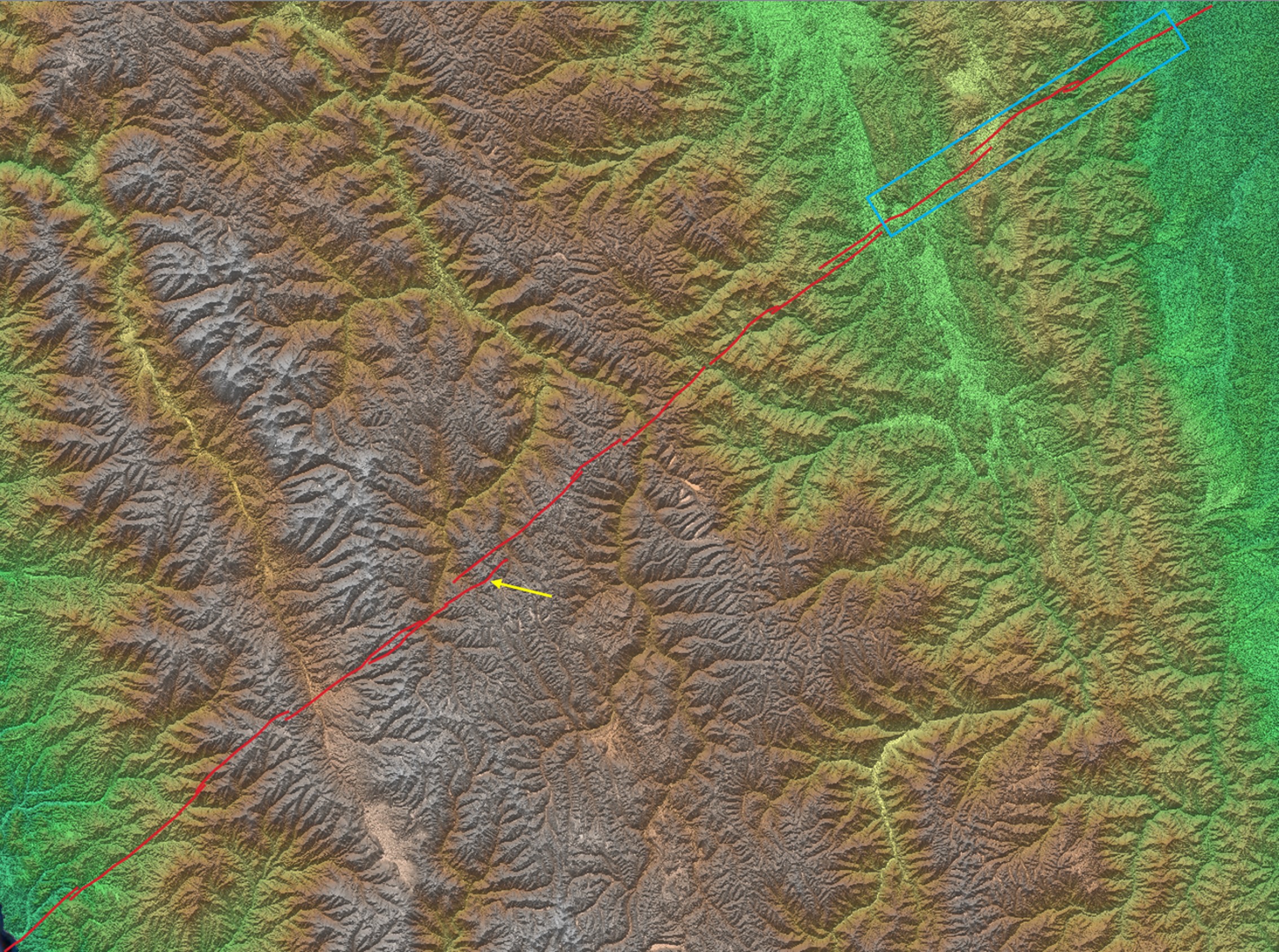
Example of NE-SW striking transcrustal structure, along which Potosí has been emplaced
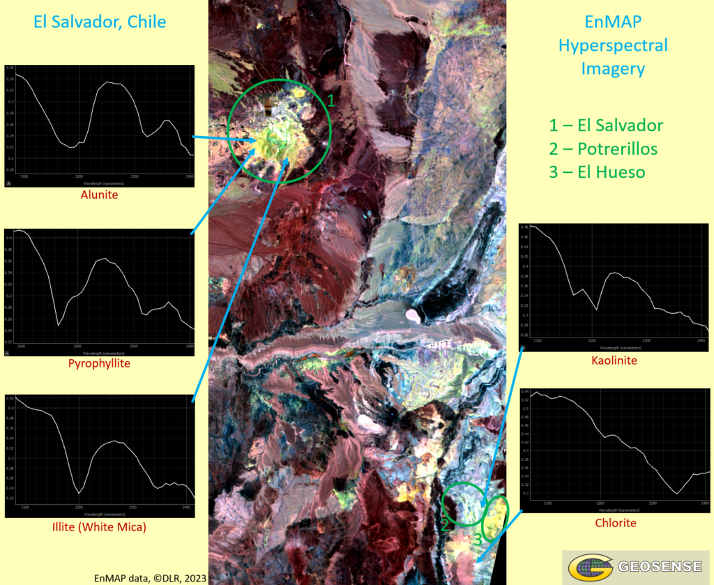
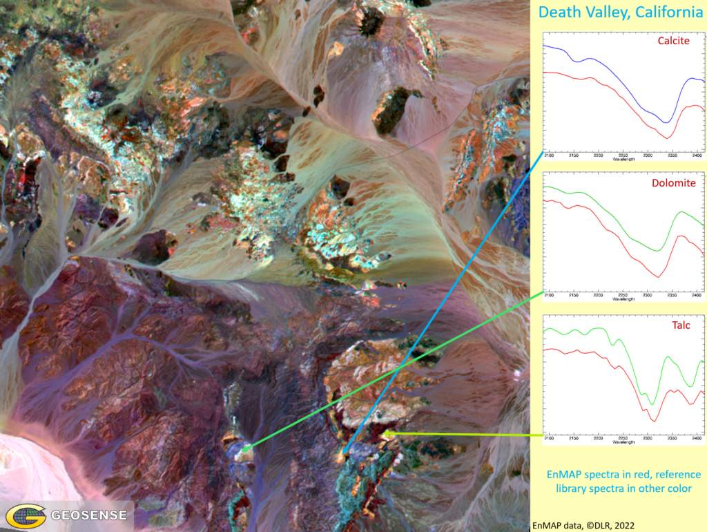
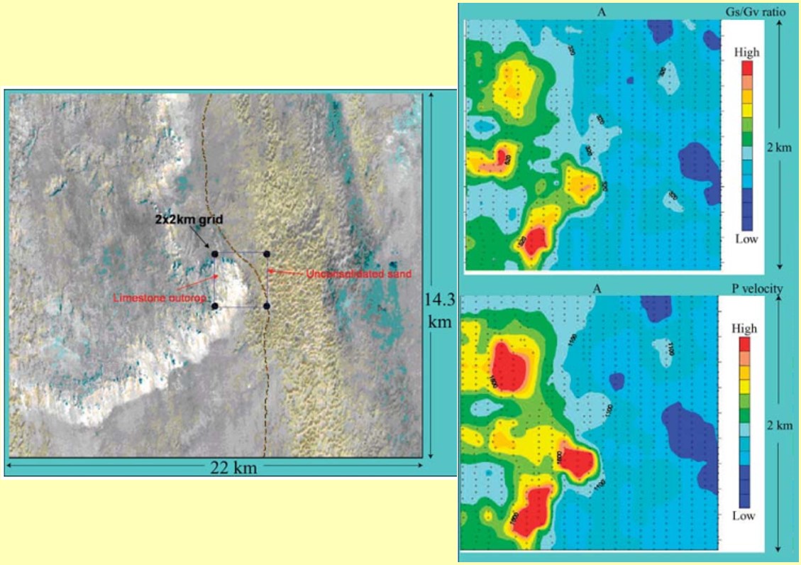
There are other benefits of applying geological remote sensing during the outside-in exploration workflow. Where exposure of rocks at surface is good enough, geological remote sensing techniques make it possible to recognize the locations that show evidence of significant fluid flow, by mapping hydrothermal alteration. This information can be particularly relevant when making the camp-scale decision, and attempting to select the ground with the highest probability of hosting an ore body (at least for those deposit types that have a recognizable alteration halo).
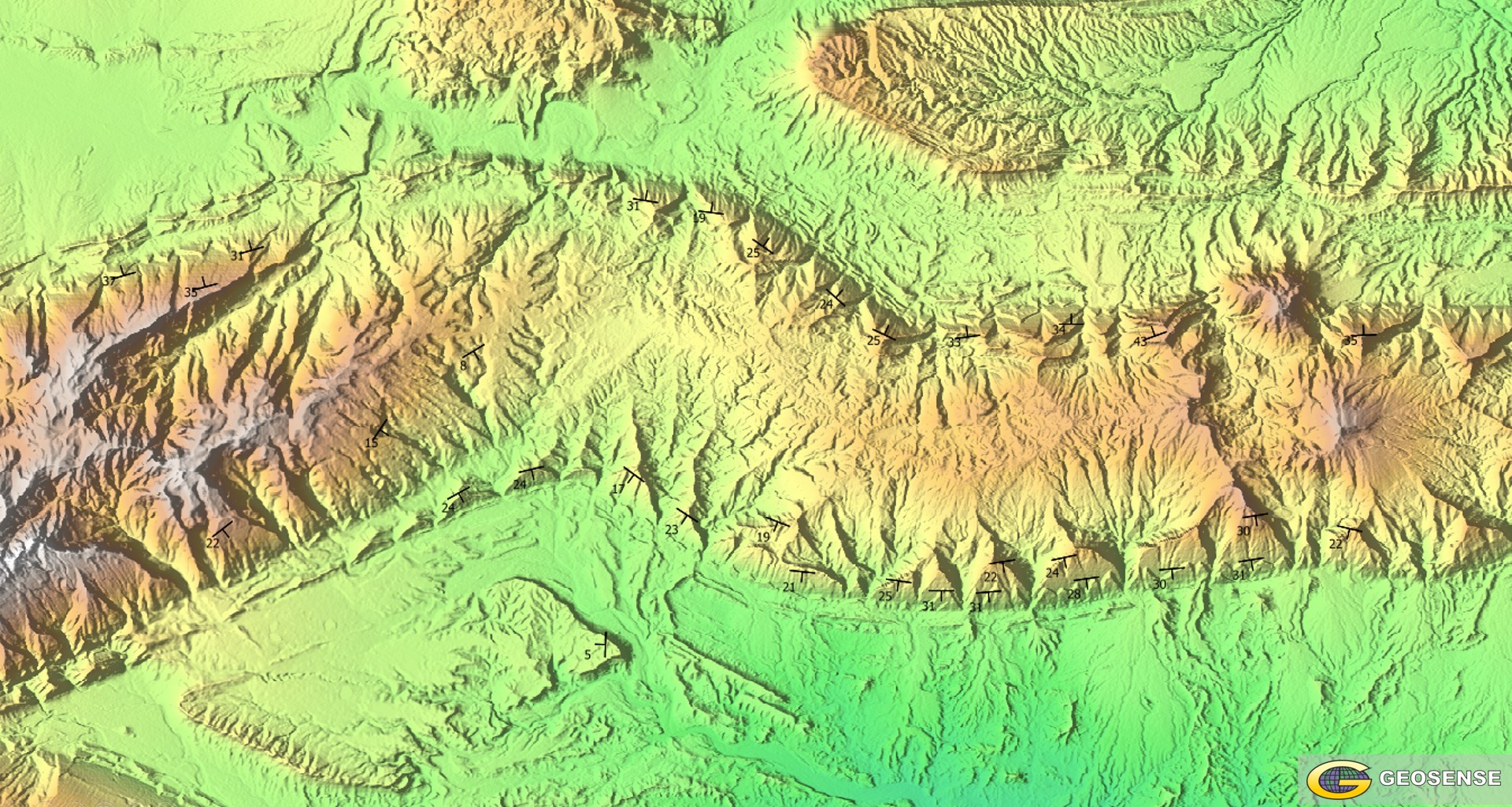
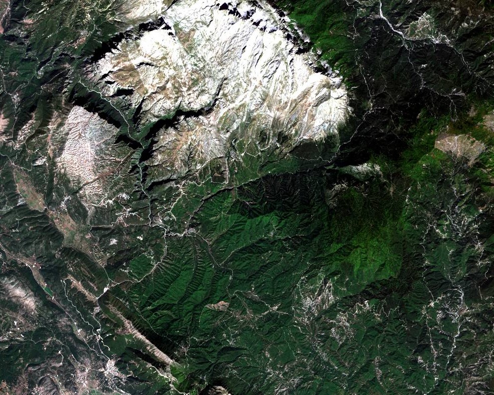
Once the initial regional mapping work has been done, and the camp-scale decision has been made there are higher resolution imagery and elevation datasets that enable us to map key aspects of the geology in significantly more detail. This includes commercial datasets that have a significantly higher spatial resolution, but are otherwise consistent with the free, lower resolution datasets used before. These datasets enable more detailed mapping of the structural geology, alteration and stratigraphy, within areas that were selected during the previous phase of the outside-in exploration workflow. This mapping phase is an ideal preparation for fieldwork, to ensure the precious time of field geologists is spent in the right locations.
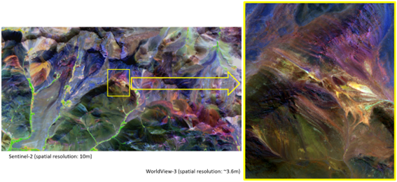
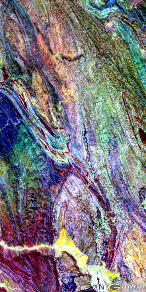
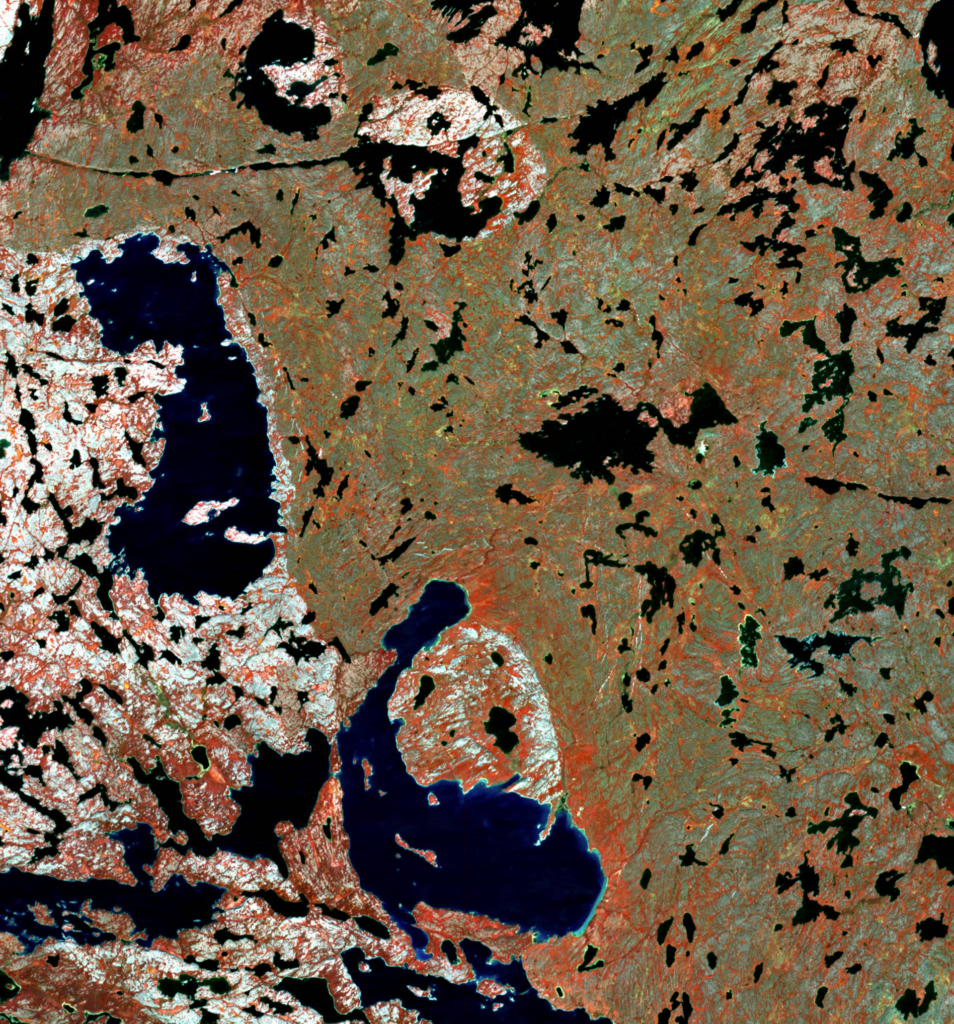
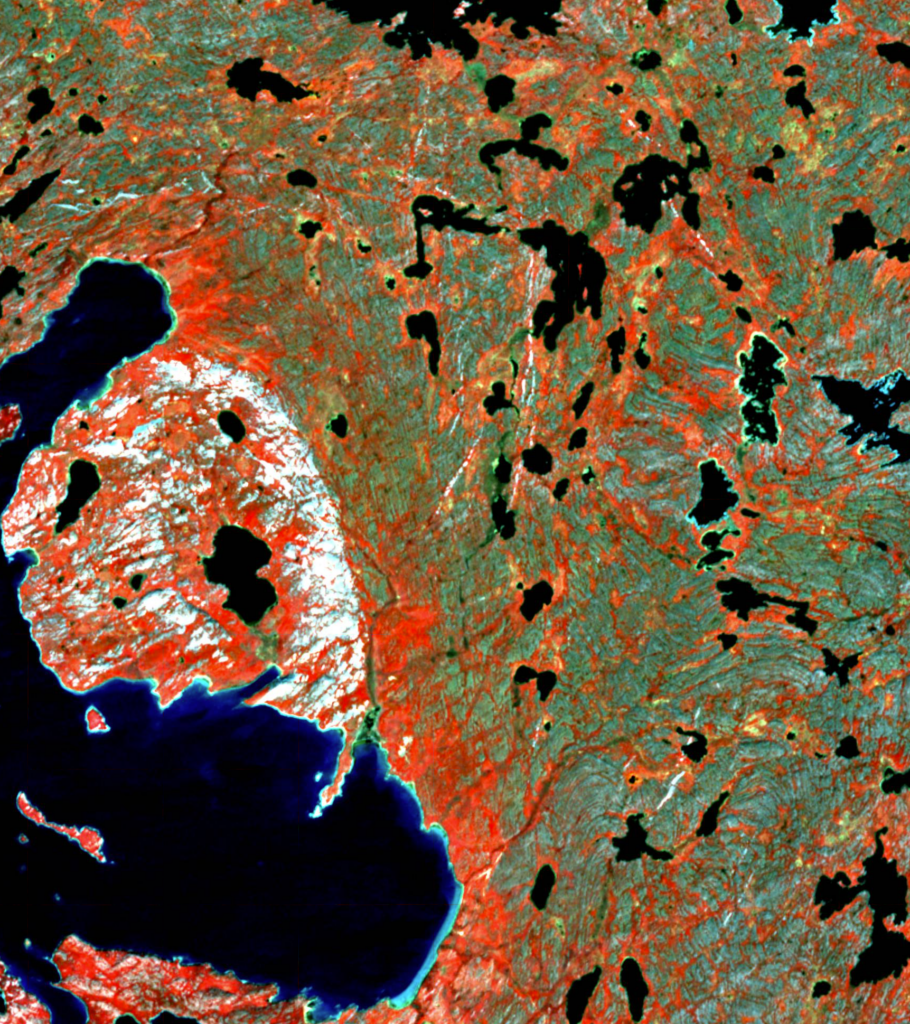
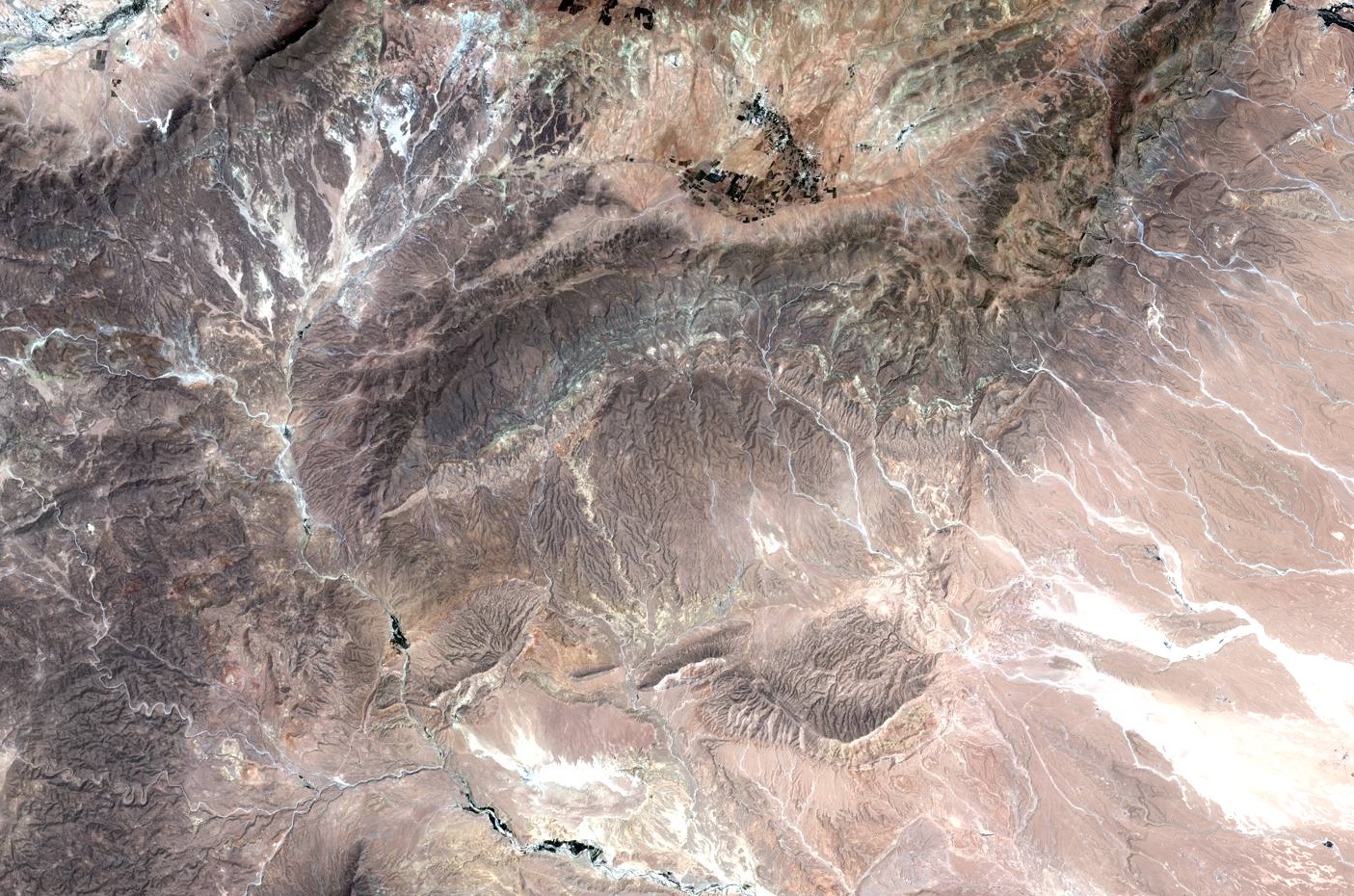
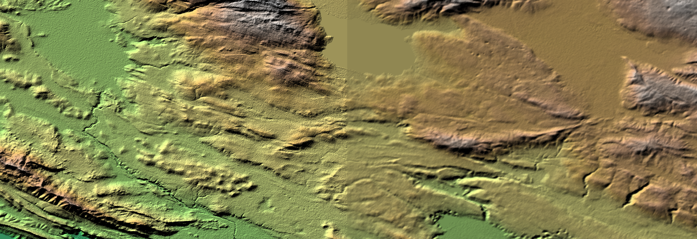
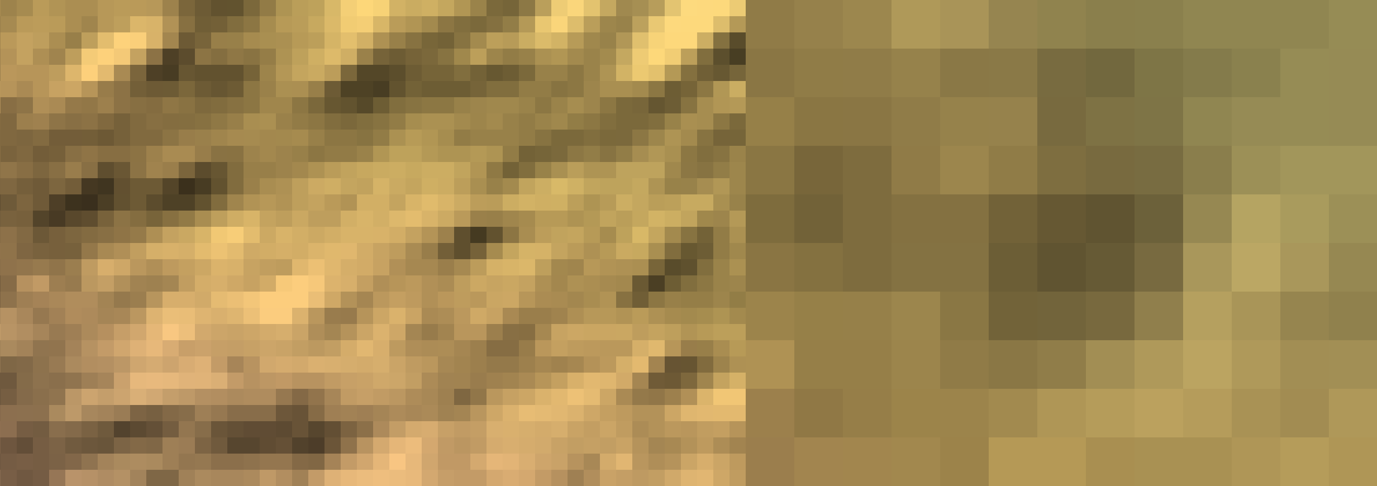
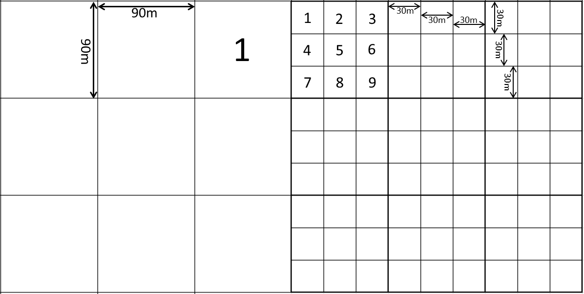
Color composites of different multispectral images, with similar spectral bands. Both datasets are consistent across different scale, and as a result, ideal for use during subsequent phases of an outside-in exploration workflow
This part of the outside-in exploration workflow is where the majority of Jun Cowan’s work is focused, and where he mostly applies the outside-in approach; from the regional (district/camp) scale, down to the deposit scale. He specializes in recognizing structural patterns in assay data from drill holes, and regularly shares valuable insights about repeated patterns that he observes when working with these datasets.
Boots on the ground
In this article, we will not write much about the next stages of the exploration workflow, once boots are on the ground. The exploration activities from this moment onward continue to be very important for making discoveries. But these activities are quite well known, because the majority of geologists who work in exploration focus on the final phases of the outside-in exploration workflow (field mapping, sampling and drilling).
While an ability to differentiate minerals with a hand lens is a useful skill, once you put boots on the ground (and during drilling), it will generally not help an exploration team before that stage, when the most prospective ground needs to be selected. Mapping crustal scale structures does help improve this key phase, early on in the exploration workflow. Where possible, this type of regional structural mapping should be combined with mineral mapping, to detect subtle/cryptic alteration systems. Particularly now, after the increasing availability of high-quality hyperspectral imagery has opened up a new search space. These datasets allow us to map common alteration minerals, which could not be recognized by the multispectral imagery that were previously used for this purpose.
If you are part of an exploration team, and you want to make world class discoveries, some of the recent, big success stories should be a guide. Major discoveries like Oyu Tolgoi, Fruta del Norte, Nova-Bollinger, Kamoa-Kakula and the Vicuña District (Filo del Sol and its neighbor Lunahuasi), were not found by exploring inside-out. This was all done by systematically moving through different scales, outside-in. By starting from a concept of why an area was overlooked, and spending money on understanding relevant aspects of the geological setting at each scale. Finally, the companies put several drill holes into the targets that came out of this process, and were rewarded.
To be successful as an explorer, figure out at which projects new ideas can really be tested, and at which projects the company will mostly drill minor step-outs at targets that didn’t work in previous cycles. Understand how to apply an outside-in approach to exploration (ideally in new search spaces), which junior companies are doing this, and avoid just reworking old ‘advanced projects’. With each cycle that a project has seen significant work, the odds of a world class discovery get lower.
References
Begg, G.C., Hronsky, J., Arndt, N.T., Griffin, W.L., O’Reilly, S.Y. & Hayward, N. (2010). Lithospheric, Cratonic, and Geodynamic Setting of Ni-Cu-PGE Sulfide Deposits. Economic Geology. 105, pp. 1057 – 1070.
Cowan, E.J. (2020). Deposit-scale structural architecture of the Sigma-Lamaque gold deposit, Canada—insights from a newly proposed 3D method for assessing structural controls from drill hole data. Mineralium Deposita 55, pp. 217-240.
Groves, D.I. & Santosh, M. (2020). Craton and thick lithosphere margins: The sites of giant mineral deposits and mineral provinces. Gondwana Research. 100, pp. 195-222.
Hoggard, M.J., Czarnota, K., Richards, F.D., Huston, D.L., Jaques, A.L. & Ghelichkhan, S. (2020). Global distribution of sediment-hosted metals controlled by craton edge stability. Nature Geoscience. 13, pp. 504-510.
McCuaig, T., Beresford, S. & Hronsky, J. (2010). Translating the mineral systems approach into an effective exploration targeting system. Ore Geology Reviews. 38, pp. 128-138.
McCuaig, T. & Hronsky, J. (2014). The mineral system concept: The key to exploration targeting. Society of Economic Geologists Special Publication. 18, pp. 153-175.
A slightly edited version of this article has been published on LinkedIn.